how to draw a direction field

8.2: Direction Fields and Numerical Methods

Concluding updated
Salve as PDF

Page ID: 2557

Professor (Mathematics) at Massachusetts Institute of Technology (Strang) & University of Wisconsin-Stevens Point (Herman)
Publisher/Source: OpenStax CNX

Learning Objectives

Describe the direction field for a given commencement-order differential equation.
Use a management field to draw a solution curve of a first-order differential equation.
Use Euler's Method to approximate the solution to a kickoff-guild differential equation.

For the rest of this affiliate we will focus on various methods for solving differential equations and analyzing the behavior of the solutions. In some cases it is possible to predict properties of a solution to a differential equation without knowing the actual solution. We will also study numerical methods for solving differential equations, which can be programmed by using various estimator languages or even by using a spreadsheet program, such as Microsoft Excel.

Creating Direction Fields

Management fields (also called slope fields) are useful for investigating first-gild differential equations. In detail, we consider a outset-order differential equation of the form

\[ y'=f(x,y).\nonumber\]

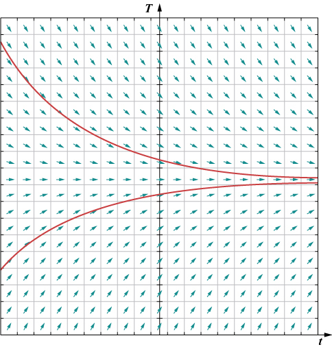
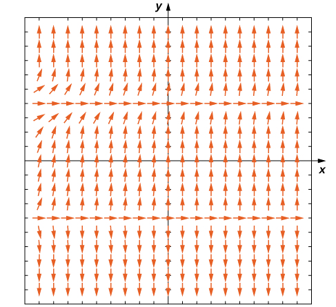
An applied example of this type of differential equation appears in Newton'southward law of cooling, which we will solve explicitly afterwards in this chapter. Start, though, let us create a direction field for the differential equation

\[ T′(t)=−0.4(T−72).\nonumber\]

Hither $ T(t)$ represents the temperature (in degrees Fahrenheit) of an object at time $ t$, and the ambience temperature is $ 72°F$. Figure $ \PageIndex{1}$ shows the direction field for this equation.

A graph of a direction field for the given differential equation in quadrants one and two. The arrows are pointing directly to the right at y = 72. Below that line, the arrows have increasingly positive slope as y becomes smaller. Above that line, the arrows have increasingly negative slope as y becomes larger. The arrows point to convergence at y = 72. Two solutions are drawn: one for initial temperature less than 72, and one for initial temperatures larger than 72. The upper solution is a decreasing concave up curve, approaching y = 72 as t goes to infinity. The lower solution is an increasing concave down curve, approaching y = 72 as t goes to infinity. — Effigy $ \PageIndex{ane}$: Management field for the differential equation $ T′(t)=−0.4(T−72)$. Ii solutions are plotted: one with initial temperature less than $ 72°F$ and the other with initial temperature greater than $ 72°F$.

The thought backside a management field is the fact that the derivative of a function evaluated at a given signal is the slope of the tangent line to the graph of that function at the same point. Other examples of differential equations for which we tin create a direction field include

\[ y'=3x+2y−four\nonumber\]

\[ y'=x^2−y^2\nonumber\]

\[ y'=\frac{2x+4}{y−ii}.\nonumber\]

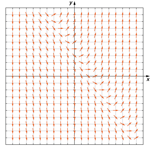
To create a management field, we kickoff with the first equation: $ y'=3x+2y−4$. We let $ \left(x_0,\, y_0\right)$ exist any ordered pair, and we substitute these numbers into the right-mitt side of the differential equation. For example, if we cull $ x=1$ and $ y=2$, substituting into the correct-hand side of the differential equation yields

$ y′=3x+2y−four=3(1)+ii(two)−4=3.$

This tells u.s. that if a solution to the differential equation $ y'=3x+2y−4$ passes through the point $ (1,ii)$, then the gradient of the solution at that point must equal 3. To starting time creating the direction field, nosotros put a short line segment at the bespeak $ (ane,two)$ having slope $ 3$. We can practice this for whatever point in the domain of the function $ f(x,y)=3x+2y−4,$ which consists of all ordered pairs $ (x,y)$ in $ R^2$. Therefore any signal in the Cartesian aeroplane has a slope associated with information technology, bold that a solution to the differential equation passes through that betoken. The direction field for the differential equation $ y′=3x+2y−4$ is shown in Figure $ \PageIndex{2}$.

A graph of the direction field for the differential equation y' = 3 x + 2 y – 4 in all four quadrants. In quadrants two and three, the arrows point down and slightly to the right. On a diagonal line, roughly y = -x + 2, the arrows point further and further to the right, curve, and then point up above that line. — Effigy $ \PageIndex{ii}$: Direction field for the differential equation $ y'=3x+2y−iv$.

We can generate a direction field of this type for any differential equation of the course $ y'=f(x,y).$

Definition: Direction Field (Gradient Field)

A direction field (slope field) is a mathematical object used to graphically represent solutions to a first-society differential equation. At each point in a direction field, a line segment appears whose slope is equal to the gradient of a solution to the differential equation passing through that indicate.

Using Direction Fields

Nosotros can employ a management field to predict the behavior of solutions to a differential equation without knowing the actual solution. For example, the direction field in Figure $ \PageIndex{3}$ serves as a guide to the behavior of solutions to the differential equation $ y'=3x+2y−iv.$

To utilize a direction field, nosotros get-go by choosing any point in the field. The line segment at that point serves every bit a signpost telling us what management to go from in that location. For example, if a solution to the differential equation passes through the signal $ (0,1),$ so the slope of the solution passing through that bespeak is given by $ y'=3(0)+2(1)−4=−2.$ Now let $ x$ increase slightly, say to $ x=0.ane$. Using the method of linear approximations gives a formula for the approximate value of $ y$ for $ ten=0.1.$ In particular,

\[ L(x)=y_0+f′(x_0)(x−x_0)=1−2(x_0−0)=1−2x_0.\nonumber\]

Substituting $ x_0=0.1$ into $ L(x)$ gives an approximate $ y$ value of $ 0.8$.

At this point the slope of the solution changes (again according to the differential equation). Nosotros can keep progressing, recalculating the slope of the solution as we take minor steps to the correct, and watching the behavior of the solution. Effigy $ \PageIndex{iii}$ shows a graph of the solution passing through the bespeak $ (0,1)$.

The curve is the graph of the solution to the initial-value problem

\[ y'=3x+2y−4,\; y(0)=1.\nonumber\]

This curve is called a solution curve passing through the point $ (0,1).$ The exact solution to this initial-value problem is

\[ y=−\frac{iii}{two}x+\frac{5}{4}−\frac{1}{iv}e^{2x},\nonumber\]

and the graph of this solution is identical to the bend in Effigy $ \PageIndex{3}$.

Exercise $\PageIndex{ane}$

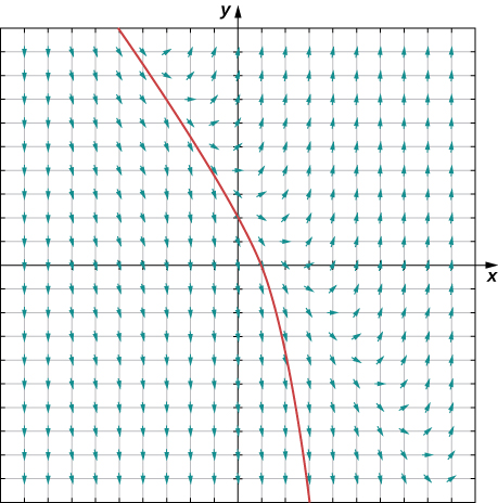
Create a direction field for the differential equation $ y'=x^2−y^2$ and sketch a solution curve passing through the point $ (−one,two)$.

Hint: Use $ x$ and $ y$ values ranging from $ −five$ to $ five$. For each coordinate pair, summate $ y'$ using the correct-paw side of the differential equation.

Answer: $A graph of the direction field for the differential equation y' = x ^ 2 – y ^ 2. Along y = x and y = -x, the lines are horizontal. On either side of y = x and y = -x, the lines slant and direct solutions along those two functions. The rest of the lines are vertical. The solution going through (-1, 2) is shown. It curves down from about (-2.75, 10), through (-1, 2) and about (0, 1.5), and then up along the diagonal to (10, 10).$

Now consider the management field for the differential equation $ y'=(x−3)(y^2−4)$, shown in Effigy $ \PageIndex{four}$. This direction field has several interesting properties. First of all, at $ y=−2$ and $ y=two$, horizontal dashes appear all the way across the graph. This means that if $ y=−2$, and then $ y'=0.$ Substituting this expression into the correct-manus side of the differential equation gives

\[ \begin{align*} (x−3)(y^two−4)&=(x−iii)((−2)^two−iv)\\[4pt]
&=(x−three)(0)\\[4pt]
&=0\\[4pt]
&=y'.\end{align*}\]

Therefore $ y=−2$ is a solution to the differential equation. Similarly, $ y=2$ is a solution to the differential equation. These are the but constant-valued solutions to the differential equation, every bit we can see from the following argument. Suppose $ y=g$ is a constant solution to the differential equation. So $ y′=0$. Substituting this expression into the differential equation yields $ 0=(x−3)(chiliad^2−4)$. This equation must be true for all values of $ x$, so the 2d cistron must equal zippo. This result yields the equation $ k^2−four=0$. The solutions to this equation are $ yard=−2$ and $ k=2$, which are the abiding solutions already mentioned. These are called the equilibrium solutions to the differential equation.

A direction field for the given differential equation. The arrows are horizontal and pointing to the right at y = -2, y = 2, and x = 3. The closer the arrows are to x = 6, the more horizontal the arrows become. The further away, the more vertical they are. — Figure $ \PageIndex{4}$: Management field for the differential equation $ y'=(x−3)(y^2−four)$ showing ii solutions. These solutions are very close together, but ane is barely above the equilibrium solution $ x=−2$ and the other is barely below the same equilibrium solution.

Definition: Equilibrium Solutions

Consider the differential equation $ y'=f(x,y)$. An equilibrium solution is whatever solution to the differential equation of the form $ y=c$, where $c$ is a constant.

To determine the equilibrium solutions to the differential equation $ y'=f(x,y)$, set up the right-mitt side equal to zero. An equilibrium solution of the differential equation is whatsoever function of the grade $ y=k$ such that $ f(x,k)=0$ for all values of $ 10$ in the domain of $ f$.

An important characteristic of equilibrium solutions concerns whether or not they arroyo the line $ y=k$ as an asymptote for large values of $ x$.

Definition: asymptotically Stable, Unstable and Semi-Stable Solutions

Consider the differential equation $ y′=f(10,y),$ and assume that all solutions to this differential equation are defined for $ x≥x_0$. Let $ y=k$ be an equilibrium solution to the differential equation.

$ y=one thousand$ is an asymptotically stable solution to the differential equation if there exists $ ε>0$ such that for any value $ c∈(k−ε,\, k+ε)$ the solution to the initial-value problem $ y′=f(x,y), \; y(x_0)=c$ approaches $ k$ as $ 10$ approaches infinity.
$ y=k$ is an asymptotically unstable solution to the differential equation if at that place exists $ ε>0$ such that for any value $ c∈(k−ε,\, k+ε)$ the solution to the initial-value trouble $ y′=f(x,y), \; y(x_0)=c$ never approaches $ chiliad$ every bit $ x$ approaches infinity.
$ y=k$ is an asymptotically semi-stable solution to the differential equation if it is neither asymptotically stable nor asymptotically unstable.

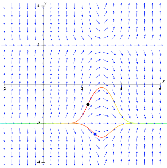
Now we return to the differential equation $ y'=(x−3)(y^ii−4)$, with the initial condition $ y(0)=0.v$. The direction field for this initial-value problem, along with the corresponding solution, is shown in Figure $ \PageIndex{5}$.

A direction field for the given differential equation. The arrows are horizontal and pointing to the right at y = -2, y = 2, and x = 3. A solution is graphed that goes through (0, 0.5) and another through the point (2, -2.2). Both curves eventually approach the line y = -2 asymptotically.. — Figure $ \PageIndex{v}$: Management field for the initial-value problem $ y'=(ten−3)(y^2−4),\; y(0)=0.5.$ A second solution curve is graphed with initial condition $(ii, -2.2)$.

The values of the solution to this initial-value problem stay between $ y=−two$ and $ y=2$, which are the equilibrium solutions to the differential equation. Furthermore, as $ x$ approaches infinity, although they initially appear to approach the line y = 2, the $ y$-coordinates clearly arroyo $ -2$. The behavior of solutions is similar if the initial value is beneath $ -2$, for case, $ y(two)=-2.2$. In this case, the solutions increase and approach $ y=-2$ as $ 10$ approaches infinity. Therefore $ y=-2$ is an asymptotically stable solution to this differential equation.

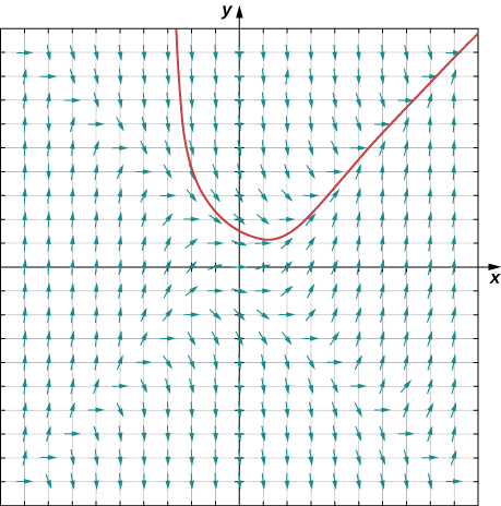
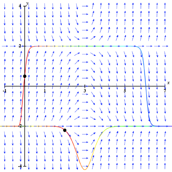
What happens when the initial value is above $ y=2$? This scenario is illustrated in Figure $ \PageIndex{half-dozen}$, with the initial value $ y(0)=3.$

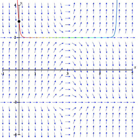
The solution increases chop-chop toward positive infinity as $ 10$ approaches infinity. Furthermore, if the initial value is slightly beneath $ ii$, and so the solution approaches $ -2$, which is the other equilibrium solution. Therefore in neither instance does the solution approach $ y=two$, so $ y=2$ is chosen an asymptotically unstable, or unstable, equilibrium solution.

Example $ \PageIndex{1}$: Stability of an Equilibrium Solution

Create a direction field for the differential equation $ y'=(y−three)^2(y^2+y−2)$ and identify any equilibrium solutions. Classify each of the equilibrium solutions equally stable, unstable, or semi-stable.

Solution

The direction field is shown in Figure $ \PageIndex{seven}$.

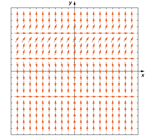
A graph of a direction field with arrows pointing to the right at y = -4, y = 2, and y = 6. For y < -iv, the arrows point upwardly. For -4 < y < 2, the arrows indicate downward. For 2 < y <6, the arrows point up, becoming flatter and flatter as they approach y = 6. For y > 6, the arrows point up and become more and more vertical the further they get from y = 6. — Effigy $ \PageIndex{vii}$: Management field for the differential equation $ y'=(y−3)^2(y^2+y−2).$

The equilibrium solutions are $ y=−2,\, y=1,$ and $ y=3$. To classify each of the solutions, look at an pointer straight above or beneath each of these values. For example, at $ y=−2$ the arrows direct below this solution point up, and the arrows directly above the solution indicate downwards. Therefore all initial conditions close to $ y=−2$ approach $ y=−2$, and the solution is stable. For the solution $ y=i$, all initial conditions in a higher place and below $ y=1$ are repelled (pushed away) from $ y=1$, so this solution is unstable. The solution $ y=3$ is semi-stable, because for initial conditions slightly greater than $ three$, the solution approaches infinity, and for initial conditions slightly less than $ 3$, the solution approaches $ y=1$.

Analysis

It is possible to notice the equilibrium solutions to the differential equation by setting the right-hand side equal to goose egg and solving for $ y.$ This arroyo gives the aforementioned equilibrium solutions as those nosotros saw in the direction field.

Do $\PageIndex{2}$

Create a management field for the differential equation $ y'=(10+v)(y+2)(y^2−4y+4)$ and identify whatever equilibrium solutions. Classify each of the equilibrium solutions equally stable, unstable, or semi-stable.

Hint: First create the direction field and expect for horizontal dashes that go all the mode across. Then examine the slope lines directly above and below the equilibrium solutions.

Respond

The equilibrium solutions are $ y=−2$ and $ y=2$. For this equation, $ y=−2$ is an unstable equilibrium solution, and $ y=ii$ is a semi-stable equilibrium solution.

$A direction field with arrows pointing to the right at y = -4 and y = 4. The arrows point up for y > -4 and downwardly for y < -4. Close to y = 4, the arrows are more horizontal, but the further away, the more vertical they become.$

Euler'due south Method

Consider the initial-value problem

\[ y′=2x−three,\;y(0)=3.\nonumber\]

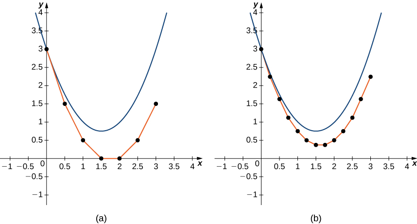
Integrating both sides of the differential equation gives $ y=ten^2−3x+C,$ and solving for $ C$ yields the particular solution $ y=10^two−3x+3.$ The solution for this initial-value trouble appears as the parabola in Figure $ \PageIndex{8}$.

A graph over the range [-1,4] for x and y. The given upward opening parabola is drawn with vertex at (1.5, 0.75). Individual points are plotted at (0, 3), (0.5, 1.5), (1, 0.5), (1.5, 0), (2, 0), (2.5, 0.5), and (3, 1.5) with line segments connecting them. — Effigy $ \PageIndex{8}$: Euler's Method for the initial-value problem $ y′=2x−three,y(0)=iii.$

The blood-red graph consists of line segments that gauge the solution to the initial-value problem. The graph starts at the same initial value of $ (0,three)$. So the slope of the solution at any point is determined past the correct-mitt side of the differential equation, and the length of the line segment is determined by increasing the $ x$ value by $ 0.5$ each fourth dimension (the step size). This approach is the ground of Euler'south Method.

Before nosotros state Euler's Method every bit a theorem, let's consider some other initial-value problem:

\[ y′=10^ii−y^ii,\; y(−1)=2.\nonumber\]

The idea behind direction fields can besides be applied to this problem to study the behavior of its solution. For case, at the point $ (−1,2),$ the slope of the solution is given by $ y'=(−1)^2−2^2=−3$, then the slope of the tangent line to the solution at that indicate is as well equal to $ −three$. Now we define $ x_0=−1$ and $ y_0=2$. Since the slope of the solution at this point is equal to $ −3$, we can use the method of linear approximation to gauge y most $ (−one,2)$.

\[ L(x)=y_0+f′(x_0)(ten−x_0).\nonumber\]

Here $ x_0=−1,y_0=2,$ and $ f′(x_0)=−iii,$ so the linear approximation becomes

\[ Fifty(ten)=2−iii(x−(−i))=two−3x−three=−3x−1.\nonumber\]

At present we cull a step size. The step size is a small value, typically $ 0.1$ or less, that serves equally an increment for $ 10$; it is represented by the variable $ h$. In our instance, let $ h=0.1$. Incrementing $ x_0$ by $ h$ gives our adjacent $ x$ value:

\[ x_1=x_0+h=−1+0.1=−0.9.\nonumber\]

We can substitute $ x_1=−0.nine$ into the linear approximation to calculate $ y_1$.

\[ y_1=L(x_1)=−3(−0.ix)−one=1.7.\nonumber\]

Therefore the gauge $ y$ value for the solution when $ x=−0.9$ is $ y=1.7$. We can then repeat the process, using $ x_1=−0.9$ and $ y_1=1.seven$ to calculate $ x_2$ and $ y_2$. The new slope is given by $ y'=(−0.9)^two−(one.7)^2=−2.08.$ First, $ x_2=x_1+h=−0.9+0.1=−0.8.$ Using linear approximation gives

$ \brainstorm{align*} L(x)&=y_1+f′(x_1)(x−x_1)\\[4pt]
&=one.7−2.08(10−(−0.ix))\\[4pt]
&=one.7−ii.08x−i.872\\[4pt]
&=−two.08x−0.172. \end{align*}$

Finally, we substitute $ x_2=−0.8$ into the linear approximation to calculate $ y_2$.

$\begin{marshal*} y_2&=L(x_2)\\[4pt]
&=−2.08x_2−0.172\\[4pt]
&=−2.08(−0.8)−0.172\\[4pt]
&=one.492.\end{align*}$

Therefore the judge value of the solution to the differential equation is $ y=1.492$ when $ x=−0.8.$

What we take just shown is the idea behind Euler'southward Method. Repeating these steps gives a list of values for the solution. These values are shown in the table, rounded off to four decimal places.

Table $ \PageIndex{1}$: Using Euler'south Method to Estimate Solutions to a Differential Equation
$ n$	0	1	2	three	4	v
$ x_n$	−1	−0.9	−0.8	−0.7	−0.vi	−0.5
$ y_n$	2	ane.7	ane.492	1.3334	1.2046	i.0955
$ northward$	half-dozen	seven	8	9	10
$ x_n$	−0.four	−0.3	−0.2	−0.i	0
$ y_n$	1.0004	1.9164	1.8414	1.7746	1.7156

Euler'due south method

Consider the initial-value trouble

\[ y'=f(x,y),\; y(x_0)=y_0.\nonumber\]

To approximate a solution to this problem using Euler's method, define

$ x_n=x_0+nh$

$ y_n=y_{n−i}+hf(x_{northward−1},y_{north−1})$.

Here $ h>0$ represents the stride size and $ n$ is an integer, starting with $ 1$. The number of steps taken is counted past the variable $ northward$.

Typically $ h$ is a small value, say $ 0.i$ or $ 0.05$. The smaller the value of $ h$, the more than calculations are needed. The college the value of $ h$, the fewer calculations are needed. Even so, the tradeoff results in a lower degree of accuracy for larger pace size, as illustrated in Figure $ \PageIndex{ix}$.

Two graphs of the same parabola, y = x ^ 2 – 3 x + 3. The first shows Euler's method for the given initial-value problem with a step size of h = 0.05, and the second shows Euler's method with a step size of h = 0.25. The first then has the points (0, 3), (.5, 1.5), (1, 0.5), (1.5, 0), (2, 0), (2.5, 0.5), and (3, 1.5) plotted with line segments connecting them. The second has the points (0, 3), (0.25, 2.25), (0.5, 1.625), (0.75, 1.125), (1, 0.75), (1.25, 0.5), (1.5, 0.375), (2, 0.5), (2.25, 0.75), (2.5, 1.125), (2.75, 1.625), and (3, 2.25) plotted with line segments connecting them. — Effigy $ \PageIndex{9}$: Euler's method for the initial-value problem $ y′=2x−three,\; y(0)=3$ with (a) a step size of $ h=0.five$; and (b) a step size of $ h=0.25.$

Example $ \PageIndex{2}$: Using Euler'south Method

Consider the initial-value problem

\[ y′=3x^ii−y^2+1,\; y(0)=2.\nonumber\]

Use Euler's method with a step size of $ 0.i$ to generate a table of values for the solution for values of $ x$ between $ 0$ and $ 1$.

Solution

We are given $ h=0.1$ and $ f(ten,y)=3x^two−y^ii+i.$ Furthermore, the initial condition $ y(0)=ii$ gives $ x_0=0$ and $ y_0=2$. Using Equation with $ north=0$, we tin generate this table.

Table $ \PageIndex{2}$: Using Euler's Method to Approximate Solutions to a Differential Equation
$ n$	$ x_n$	$ y_n=y_{n−1}+hf(x_{n−1},y_{due north−1})$
0	0	2
one	0.one	$ y_1=y_0+hf(x_0,y_0)=one.7$
two	0.2	$ y_2=y_1+hf(x_1,y_1)=1.514$
3	0.3	$ y_3=y_2+hf(x_2,y_2)=1.3968$
4	0.4	$ y_4=y_3+hf(x_3,y_3)=one.3287$
5	0.5	$ y_5=y_4+hf(x_4,y_4)=1.3001$
half dozen	0.6	$ y_6=y_5+hf(x_5,y_5)=1.3061$
7	0.7	$ y_7=y_6+hf(x_6,y_6)=i.3435$
8	0.8	$ y_8=y_7+hf(x_7,y_7)=1.4100$
9	0.9	$ y_9=y_8+hf(x_8,y_8)=1.5032$
10	one.0	$ y_{10}=y_9+hf(x_9,y_9)=1.6202$

With 10 calculations, we are able to judge the values of the solution to the initial-value problem for values of $ x$ betwixt $ 0$ and $ i$.

Go to this website for a chance to visually explore Euler's method.

Practise $\PageIndex{3}$

Consider the initial-value problem

\[ y′=x^three+y^2,\; y(one)=−two.\nonumber\]

Using a stride size of $ 0.1$, generate a table with approximate values for the solution to the initial-value problem for values of $ x$ between $ 1$ and $ 2$.

Hint: Starting time by identifying the value of $ h$, so figure out what $ f(x,y)$ is. Then employ the formula for Euler's Method to calculate $ y_1,y_2,$ and then on.

Answer

Table $ \PageIndex{3}$: Using Euler's Method to estimate solutions to the differential equation in Exercise $\PageIndex{3}$.
$ due north$	\( x_n)	$ y_n=y_{n−ane}+hf(x_{n−one},y_{due north−1})$
0	1	−2
1	one.one	$ y_1=y_0+hf(x_0,y_0)=−one.5$
2	i.2	$ y_2=y_1+hf(x_1,y_1)=−1.1419$
three	1.3	$ y_3=y_2+hf(x_2,y_2)=−0.8387$
four	1.4	$ y_4=y_3+hf(x_3,y_3)=−0.5487$
5	ane.5	$ y_5=y_4+hf(x_4,y_4)=−0.2442$
half-dozen	1.6	$ y_6=y_5+hf(x_5,y_5)=0.0993$
7	1.7	$ y_7=y_6+hf(x_6,y_6)=0.5099$
eight	1.eight	$ y_8=y_7+hf(x_7,y_7)=1.0272$
9	i.9	$ y_9=y_8+hf(x_8,y_8)=ane.7159$
x	2	$ y_{10}=y_9+hf(x_9,y_9)=2.6962$

Primal Concepts

A direction field is a mathematical object used to graphically represent solutions to a kickoff-gild differential equation.
Euler's Method is a numerical technique that tin can be used to approximate solutions to a differential equation.

Key Equations

Euler'south Method

$ x_n=x_0+nh$

$ y_n=y_{north−1}+hf(x_{n−1},y_{n−1})$, where $ h$ is the step size

Glossary

asymptotically semi-stable solution: $ y=yard$ if it is neither asymptotically stable nor asymptotically unstable

asymptotically stable solution: $ y=one thousand$ if at that place exists $ ε>0$ such that for whatever value $ c∈(k−ε,\, k+ε)$ the solution to the initial-value problem $ y′=f(x,y),\; y(x_0)=c$ approaches $ k$ as $ x$ approaches infinity

asymptotically unstable solution: $ y=chiliad$ if there exists $ ε>0$ such that for whatever value $ c∈(grand−ε,\, chiliad+ε)$ the solution to the initial-value problem $ y′=f(ten,y),\; y(x_0)=c$ never approaches $ k$ as $ x$approaches infinity

direction field (slope field): a mathematical object used to graphically correspond solutions to a first-order differential equation; at each bespeak in a direction field, a line segment appears whose slope is equal to the slope of a solution to the differential equation passing through that signal

equilibrium solution: any solution to the differential equation of the form $ y=c,$ where $ c$ is a constant

Euler'due south Method: a numerical technique used to approximate solutions to an initial-value problem

solution curve: a bend graphed in a direction field that corresponds to the solution to the initial-value problem passing through a given point in the direction field

step size: the increase hh that is added to the xx value at each step in Euler'south Method

Contributors and Attributions

Gilbert Strang (MIT) and Edwin "Jed" Herman (Harvey Mudd) with many contributing authors. This content by OpenStax is licensed with a CC-BY-SA-NC iv.0 license. Download for free at http://cnx.org.
Paul Seeburger (Monroe Community College) edited this section to adjust the explanation of equilibrium points in the instance shown in Figures $ \PageIndex{four}$ - $ \PageIndex{6}$. He also created these figures.

Source: https://math.libretexts.org/Bookshelves/Calculus/Book%3A_Calculus_(OpenStax)/08%3A_Introduction_to_Differential_Equations/8.2%3A_Direction_Fields_and_Numerical_Methods

Posted by: rutledgepaus1952.blogspot.com

how to draw a direction field

8.2: Direction Fields and Numerical Methods

Creating Direction Fields

Using Direction Fields

Euler'due south Method

Primal Concepts

Key Equations

Glossary

Contributors and Attributions

0 Response to "how to draw a direction field"

Post a Comment

Iklan Atas Artikel

Iklan Tengah Artikel 1

Iklan Tengah Artikel 2

Iklan Bawah Artikel

\( n\)	0	1	2	three	4	v
\( x_n\)	−1	−0.9	−0.8	−0.7	−0.vi	−0.5
\( y_n\)	2	ane.7	ane.492	1.3334	1.2046	i.0955
\( northward\)	half-dozen	seven	8	9	10
\( x_n\)	−0.four	−0.3	−0.2	−0.i	0
\( y_n\)	1.0004	1.9164	1.8414	1.7746	1.7156

\( n\)	\( x_n\)	\( y_n=y_{n−1}+hf(x_{n−1},y_{due north−1})\)
0	0	2
one	0.one	\( y_1=y_0+hf(x_0,y_0)=one.7\)
two	0.2	\( y_2=y_1+hf(x_1,y_1)=1.514\)
3	0.3	\( y_3=y_2+hf(x_2,y_2)=1.3968\)
4	0.4	\( y_4=y_3+hf(x_3,y_3)=one.3287\)
5	0.5	\( y_5=y_4+hf(x_4,y_4)=1.3001\)
half dozen	0.6	\( y_6=y_5+hf(x_5,y_5)=1.3061\)
7	0.7	\( y_7=y_6+hf(x_6,y_6)=i.3435\)
8	0.8	\( y_8=y_7+hf(x_7,y_7)=1.4100\)
9	0.9	\( y_9=y_8+hf(x_8,y_8)=1.5032\)
10	one.0	\( y_{10}=y_9+hf(x_9,y_9)=1.6202\)

\( due north\)	\( x_n)	\( y_n=y_{n−ane}+hf(x_{n−one},y_{due north−1})\)
0	1	−2
1	one.one	\( y_1=y_0+hf(x_0,y_0)=−one.5\)
2	i.2	\( y_2=y_1+hf(x_1,y_1)=−1.1419\)
three	1.3	\( y_3=y_2+hf(x_2,y_2)=−0.8387\)
four	1.4	\( y_4=y_3+hf(x_3,y_3)=−0.5487\)
5	ane.5	\( y_5=y_4+hf(x_4,y_4)=−0.2442\)
half-dozen	1.6	\( y_6=y_5+hf(x_5,y_5)=0.0993\)
7	1.7	\( y_7=y_6+hf(x_6,y_6)=0.5099\)
eight	1.eight	\( y_8=y_7+hf(x_7,y_7)=1.0272\)
9	i.9	\( y_9=y_8+hf(x_8,y_8)=ane.7159\)
x	2	\( y_{10}=y_9+hf(x_9,y_9)=2.6962\)