

How To Arbitrarily Label Draws In R
How to make bar graphs using ggplot2 in R
You can download this post as a PDF or RMarkdown file . These formats back up code highlighting.
We recently wrote nigh how IDinsight strives to use the right analytical and statistical tools to advise conclusion-makers and amend social bear on. In that post, we highlighted the benefits of the statistical software R, which is especially useful to visually communicate complex ideas. This post aims to provide beginner practitioners with the tools to make a graphic using ggplot2, a package inside R.
At the terminate of this postal service, we promise you will have a better understanding of the graph design procedure from showtime (deciding the elements of your graph) to stop (making the final graph look polished). Additionally, y'all will have code for a plot that you tin can easily modify for your futurity graphing needs.
Motivation
There is a wealth of data on the philosophy of ggplot2, how to get started with ggplot2, and how to customize the smallest elements of a graphic using ggplot2 — but it's all in different corners of the Net. Information technology can be difficult for a beginner to tie all this information together.
Prerequisites
This post assumes basic familiarity with the following R concepts:
• vectors
• data frames
• factors
I also use the dplyr package to make clean data. All code is commented so this should be straightforward to follow even if y'all have not used dplyr before.
Data
We volition be using the GapMinder dataset that comes pre-packaged with R. This dataset is an extract from the GapMinder data, and it shows the life expectancy, population and Gdp per capita of various countries over 12 years between 1952 to 2007.
                      ## # A tibble: 6 10 6
            ##   country     continent  year lifeExp      pop gdpPercap
            ##   <fct>       <fct>     <int>   <dbl>    <int>     <dbl>
            ## 1 Afghanistan Asia       1952    28.8  8425333      779.
            ## 2 Transitional islamic state of afghanistan Asia       1957    30.3  9240934      821.
            ## 3 Transitional islamic state of afghanistan Asia       1962    32.0 10267083      853.
            ## 4 Transitional islamic state of afghanistan Asia       1967    34.0 11537966      836.
            ## 5 Transitional islamic state of afghanistan Asia       1972    36.1 13079460      740.
            ## 6 Afghanistan Asia       1977    38.4 14880372      786.
Visualization task
We would like to prove the modify in life expectancy from 1952 to 2007 for 11 (arbitrarily-selected) countries: Bolivia, China, Ethiopia, Guatemala, Haiti, India, Kenya, Pakistan, Sri Lanka, Tanzania, Uganda.
Specifically, we want to see the life expectancy in each of these countries in 1952 and 2007. We also want to grouping the countries by continent.
We volition use a bar plot to communicate this information graphically because nosotros can easily see the levels of the life expectancy variable, and compare values over time and across countries. Here is a rough sketch to get u.s. started on what we can do:
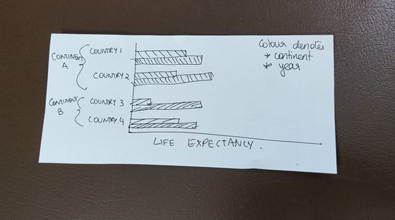
Note that nosotros want 2 bars per country — one of these should be the life expectancy in 1952 and the other in 2007. Nosotros also desire to colour the bars differently based on the continent.
Components of the graph
ggplot2 is based on the "grammar of graphics", which provides a standard mode to describe the components of a graph (the "gg" in ggplot2 refers to the grammer of graphics). It has specialized terminology to refer to the elements of a graph, and I'll innovate and explain new terms every bit we run across them. For now, what nosotros need to understand is that we volition build a graphic by calculation components one afterwards the other, like layers.
The outset step to building the graphic is to identify the components. Using our rough sketch as a guide, we know that our components are:
- Dataset — for us, this is a subset of the gapminder data that includes only the countries and years in question
- Coordinate organization — Cartesian
- Axes — nosotros want country name on the x-axis and life expectancy on the y-axis
- Type of visualization — we desire one bar per country per year e.g. for Bharat, nosotros want one bar for the life expectancy in 1952 and another bar for 2007
- Groups on the x-axis — we desire to group countries past continent
Now that we know what we need to include in the graph, allow's move on to writing code.
Making the chart
Setup
We need to install the post-obit packages:
-
ggplot2 -
dplyr— to dispense information -
gapminder— data source
We can use the following code to install and load packages.
# create list of packages we need
packages <- c("ggplot2", "dplyr", "gapminder")# Install packages
lapply(packages, install.packages, graphic symbol.only = True)# Load packages
# In case you are unfamiliar with lapply() - it has been used to employ the install.packages() and library() functions over a listing of package names. More information here: https://www.r-bloggers.com/using-apply-sapply-lapply-in-r/
lapply(packages, library, character.but = Truthful)
Manipulating the data
Let's have a look at the data once more. Information technology'due south saved nether gapminder:
          caput(gapminder)                      ## # A tibble: 6 x six
            ##   country     continent  year lifeExp      pop gdpPercap
            ##   <fct>       <fct>     <int>   <dbl>    <int>     <dbl>
            ## one Afghanistan Asia       1952    28.8  8425333      779.
            ## 2 Afghanistan Asia       1957    thirty.iii  9240934      821.
            ## 3 Afghanistan Asia       1962    32.0 10267083      853.
            ## iv Afghanistan Asia       1967    34.0 11537966      836.
            ## 5 Afghanistan Asia       1972    36.one 13079460      740.
            ## vi Afghanistan Asia       1977    38.4 14880372      786.
Permit's restrict the information to the countries and years nosotros are interested in, and save this new dataset as data_graph.
# create vectors with state names and years
country_list <- c("Republic of bolivia", "Cathay", "Federal democratic republic of ethiopia", "Republic of guatemala", "Haiti", "India", "Republic of kenya", "Pakistan", "Sri Lanka", "Tanzania", "Uganda")
year_list <- c(1952, 2007) # salvage subset of gapminder every bit data_graph
data_graph <- gapminder %>%
filter(country %in% country_list) %>%
filter(yr %in% year_list)# accept a expect at the information
## # A tibble: six 10 half dozen
head(data_graph)
## state continent yr lifeExp pop gdpPercap
## <fct> <fct> <int> <dbl> <int> <dbl>
## 1 Bolivia Americas 1952 twoscore.4 2883315 2677.
## 2 Republic of bolivia Americas 2007 65.6 9119152 3822.
## 3 China Asia 1952 44 556263527 400.
## 4 China Asia 2007 73.0 1318683096 4959.
## five Ethiopia Africa 1952 34.one 20860941 362.
## vi Ethiopia Africa 2007 52.9 76511887 691.
Let's as well make "year" a gene, since it is a discrete variable:
          data_graph <- data_graph %>%
            mutate(twelvemonth = factor(year))
Base plot
To build a ggplot, we first use the ggplot() role to specify the default data source and artful mappings:
# make the base plot and save it in the object "plot_base"
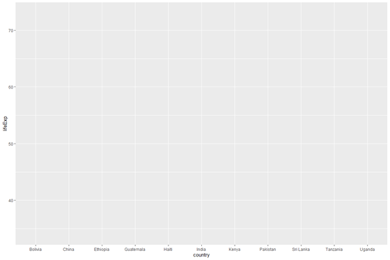
plot_base <- ggplot(information = data_graph, mapping = aes(10 = country, y = lifeExp)) # brandish the plot object
plot_base
Let'due south break this down a niggling:
- data source: "data_graph" in our case
- aesthetic mappings: The
aes()function maps variables in our information frame to aesthetic attributes. An "aesthetic attribute"" is a visual chemical element of the graph, such as the shape of a signal or the colour of a line. In our instance, nosotros are specifying that the axes (which are aesthetic attributes) should stand for to the variables "country" and "lifeExp".
Note that there is no bar graph because we haven't specified one yet. We have just specified which dataset and axes to use, not the type of graphic to brandish.
Change the appearance
Let's make the graph look a fleck nicer. My preference is to make the following adjustments:
- Simple, black-and-white layout
- No background colour
- No gridlines
- The chart surface area shouldn't be in a box; we should have only the x and y axis
We will use the theme() function to make these changes. theme() allows us to modify the display of non-information elements of the graph.
# save a better-formatted version of the base plot in "plot_base_clean"
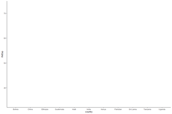
plot_base_clean <- plot_base +
# apply basic black and white theme - this theme removes the background colour past default
theme_bw() +
# remove gridlines. panel.filigree.major is for vertical lines, console.grid.minor is for horizontal lines
theme(console.grid.major = element_blank(), console.filigree.minor = element_blank(),
# remove borders
panel.border = element_blank(),
# removing borders also removes x and y axes. Add them dorsum
centrality.line = element_line()) # brandish the plot object
plot_base_clean
Notation that we did not have to re-write the code to brand the base plot or alter it in whatsoever manner. Instead, nosotros kept the base plot object as-is and "added" themes to it using the + operator. This is how we build a ggplot — we add components together to build a graphic.
Add confined
In order to add bars to our ggplot, we need to understand geometric objects ("geoms"). A "geom" is a marking we add together to the plot to represent information. For instance, we can use the geom "point" to brandish our data using points, in which case the resulting graphic would exist a scatterplot. The ggplot2 cheatsheet has a list of all the geoms nosotros can add to a plot.
We will be adding bars to our graph using geom_bar():
plot_base_clean + geom_bar(stat = "identity") 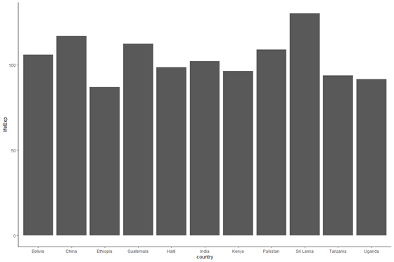
We now have a bar graph. The numbers don't seem to be right since the life expectancy is close to 100 for all countries — nosotros volition fix this subsequently.
It may seem foreign that we didn't specify the x and y values for the bars, but the bars displayed life expectancy by country anyway. This is because of ggplot'due south "bureaucracy of defaults". Since we add the call to geom_bar() to an existing telephone call to ggplot(information = data_graph, aes(x = country, y = lifeExp)), ggplot2 assumes that the x and y variables for geom_bar() are the same equally those for ggplot() i.eastward. the 10 and y variables are "state" and "lifeExp", respectively.
Nosotros besides specified stat in the call to geom_bar. stat is used when we desire to utilise a statistical part to the data and show the results graphically. When we employ geom_bar(), by default, stat assumes that nosotros want each bar to bear witness the count of y-variables per 10-variable. Since we want ggplot to plot the values as-is, we specify stat = "identity".
Modify the bar colours
Now, let'due south change the colour of the bars. Nosotros ultimately want the color of the bars to vary by continent, but allow'south start with something simpler — let's modify the colour of the bars to light blueish. To do this, we will specify fill = "lightblue" inside the telephone call to geom_bar().
plot_base_clean + geom_bar(stat = "identity", fill up = "lightblue") 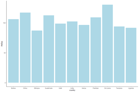
Now, let's brand the color of the bars vary by continent. Nosotros are saying that nosotros desire a mapping from an artful element (the color inside the bars) to a variable in our information ("continent"). Recall that we apply the aes() function to specify a relationship betwixt a visual chemical element and a variable. Within aes(), we volition employ the fill argument to specify that we are interested in changing the colour of the bars.
plot_base_clean + geom_bar(stat = "identity", aes(make full = continent)) 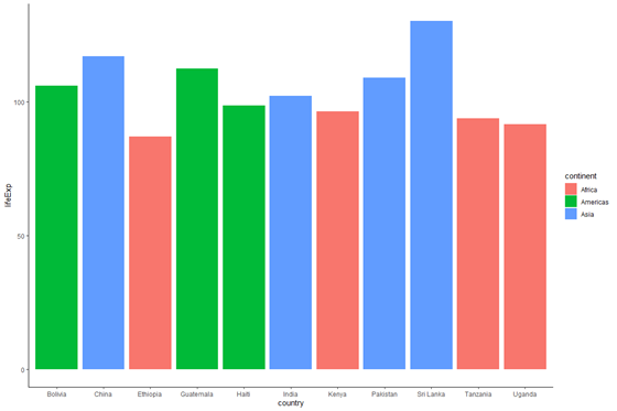
Note that we used fill in both cases, because fill is what controls the colour inside the bars. Nonetheless, nosotros did not use aes() when nosotros coloured the bars light bluish because the color within the confined wasn't related to whatever variables.
Add years
Now, we will address why we aren't seeing the correct values of life expectancy in the graph. Since each country has two observations for life expectancy (ane for 1952 and one for 2007), and we oasis't specified which observation to employ, the life expectancy shown by the bars is actually the sum of life expectancy for both years.
Permit's see what happens when nosotros restrict the graph to include but data for 2007.
          plot_base_clean +
geom_bar(information = subset(data_graph, yr == 2007), stat = "identity", aes(make full = continent)) 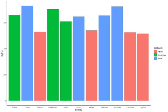
We at present meet the right values of life expectancy. Note that though the plot_base_clean object already had a default value of data (data_graph), we were able to override it in the call to geom_bar(). This again ties back to the hierarchy of defaults - if we don't specify a new dataset or xy-variables for our geoms, we simply employ the dataset and xy-variables provided in the phone call to ggplot(), but since nosotros specified a new value of information within geom_bar(), the bars reverberate a new data source.
Next, we are interested in showing 2 data points per country, one for 1952 and one for 2007. Here is where the alpha artful is useful. It specifies the transparency of the colours we are using. Allow'south try using alpha with the same subsetted dataset:
          plot_base_clean +
geom_bar(data = subset(data_graph, twelvemonth == 2007), stat = "identity", aes(make full = continent), alpha = .4) 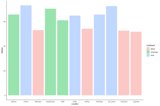
We see that similar to specifying fill = "lightblue", specifying alpha to be a number changes the transparency levels of each bar. alpha values range from 0 to 1, with higher values being more opaque.
Like make full, alpha can besides be used as an aesthetic. Let'southward establish a relationship between the transparency of a bar and the year. Since we are interested in both years, we won't restrict graph_data in geom_bar().
          plot_base_clean +
geom_bar(stat = "identity", aes(fill = continent, alpha = year)) 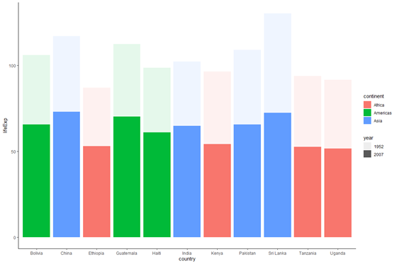
We don't want a stacked bar chart, only alpha does seem to be working - we see that the lighter portions of the bars correspond to the values in 1952, while the darker portions correspond to values in 2007.
Now, allow's use the position argument to make the bars appear side-by-side, instead of being stacked. Co-ordinate to the ggplot2 documentation, bars are stacked past default and we need to specify position = "dodge" to make the confined appear side-past-side.
          plot_base_clean +
geom_bar(stat = "identity", aes(fill = continent, alpha = year), position = "dodge") 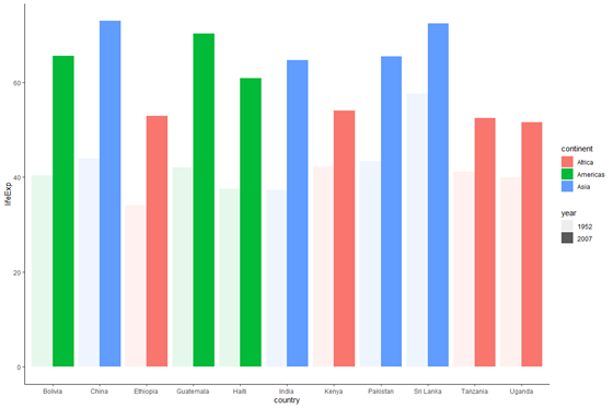
Notation that position = "dodge" is another way of writing position = position_dodge(). position_dodge() tin can take a width argument, which is discussed in detail in this Stack Overflow post. We are using the default width, which is why nosotros tin utilize the shorter version position = "contrivance".
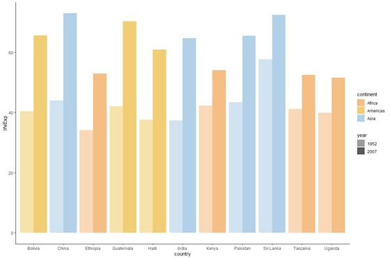
Finalize colour scheme
The 1952 colours for alpha are very light. Let'southward alter the transparency provided by blastoff using scale_alpha_manual().
          plot_base_clean +
            geom_bar(stat = "identity", aes(make full = continent, alpha = year), position = "dodge") +
scale_alpha_manual(values = c(0.6, 1)) 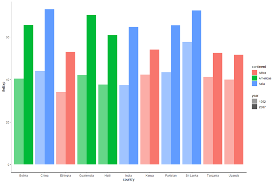
Here, we specified a vector for scale_alpha_manual, where each element provides the transparency of the corresponding twelvemonth. We assigned a transparency of 0.six to 1952 and one to 2007 (nosotros know the start element corresponds to 1952 and the second element to 2007 because that is the order of levels for the "year" gene. You lot tin can check this using levels(data_graph$year)).
Let's also change the colour scheme for the continent colours using scale_fill_manual(). We provide a vector of colours, where each chemical element provides the colour for the corresponding continent. I have provided the colours in hexadecimal format (e.thou. as "#FF0011"), just you tin provide colours in any other format you prefer.
          # add confined and colour scheme
            plot_bar <- plot_base_clean +
            geom_bar(stat = "identity", aes(fill = continent, alpha = year), position = "contrivance") +
            scale_fill_manual(values = c("#F4BE85", "#F1CE75", "#B2D1E8")) +
            scale_alpha_manual(values = c(0.six, i))               # display the plot object
              plot_bar
Make the plot horizontal
Let'south turn our plot into a horizontal bar chart using coord_flip():
          # make the plot horizontal
            plot_horizontal <- plot_bar + coord_flip()               # display the plot object
              plot_horizontal

Note the guild of the confined still reflects the levels of the factor i.e. countries coming first alphabetically are closer to the origin, and the bar for 1952 is beneath the bar for 2007. We are going to go ahead with this order, merely if you lot'd like the countries or years to announced in a different order, all y'all have to exercise is change the cistron levels of the corresponding variables.
Add facets (continent groups)
Our graph is already quite informative — we can identify the continent a country belongs to by the colour of the bar. If we want the land confined to announced by continent, nosotros tin can modify the levels of the "country" factor so that the country names are sorted by continent.
Notwithstanding, it would be much more effective if we could grouping the countries into continents on the ten-axis. The reader of the graph wouldn't need to continue referring to the legend; all the information would be in ane place. We can create these groups using facets.
Facets are used to split the ggplot into a matrix of panels. Let's add a facet for the "continent" variable to sympathize what "matrix of panels" means:
          plot_horizontal +
facet_grid(rows = vars(continent)) 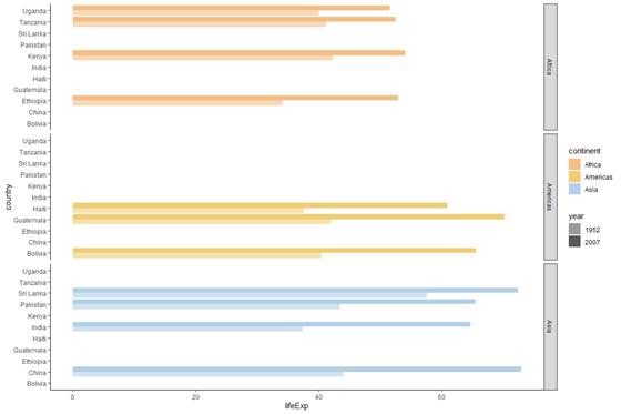
We come across that our graph is at present in 3 horizontal panels, with each console representing a different continent.
Let's pause the facet_grid() command down a little: we wanted horizontal panels, and so we specified the rows statement. Each row/console was on the ground on continent, so nosotros specified rows = vars(continent)). vars but indicates that the "continent" object exists in the context of the dataset we are using in our ggplot() command. If nosotros don't specify vars, we will get an fault saying that the object "continent" was not found.
Now, we will explore some arguments of facet_grid() that tin can improve the advent of the graph. All of these are covered in detail in the ggplot2 documentation; in this post, we will use only a few options.
First, we see that the graph is assuming that every 10-variable ("country", in our example) exists for every faceting variable ("continent") due east.chiliad. Haiti is in the Africa and Asia panel too equally the Americas panel. This is because ggplot2 assumes every panel volition take the aforementioned scale, where "scale" refers to the values the x and y centrality take on. Our calibration of interest is country names, and currently each continent has exactly the same scale - all of the country names are included for each continent. To remedy this, nosotros specify scales = "free_y" - we say that every faceting variable ("continent") can have its own scale (where a "calibration" would be merely those land names that are function of the continent).
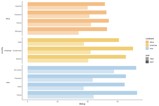
          plot_horizontal +
facet_grid(rows = vars(continent), scales = "free_y") 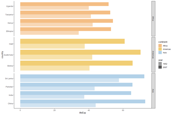
Now, notice that the bars for the Americas are thicker than the bars for Africa or Asia. This is because past default, ggplot makes all panels (i.e. all continents) occupy the same amount of space. Nosotros'd prefer that all our bars exist equally thick, rather than our panels be every bit alpine. Allow's add infinite = "free_y".
          plot_horizontal +
facet_grid(rows = vars(continent), scales = "free_y", space = "free_y") 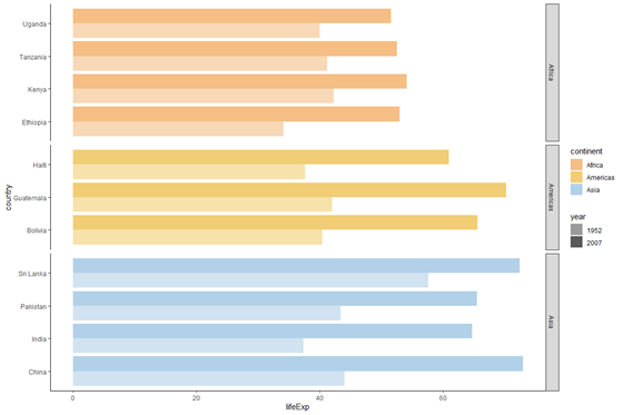
It seems a piffling confusing to have the continent names to the right and the country names to left. We tin can use the switch option to change where the facet labels (i.e. continent names) are displayed.
          # add together facets and modify their advent
            plot_facet <- plot_horizontal +
            facet_grid(rows = vars(continent), scales = "free_y", space = "free_y", switch = "y")               # display the plot object
              plot_facet
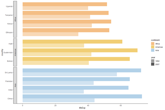
This looks quite good! Let's do the following to alter the appearance of the facet labels i.e. the continent names:
- Move the continent names to the left of country names
- Remove the gray background and box from the continent labels
- Make the continent names horizontal and non vertical
          # Modify the appearance of facet labels
            plot_facet_clean <- plot_facet +
            # motion facet characterization exterior the chart area i.e. continent names should be to the left of land names
            theme(strip.placement = "outside",
            # remove background colour from facet labels
            strip.background  = element_blank(),
            # remove border from facet label
            panel.border = element_blank(),
            # make continent names horizontal
            strip.text.y = element_text(angle = 180))               # display the plot object
              plot_facet_clean
Terminal touches
Our graph is almost ready! Let's clean upward the legend and the axes, and give a title to our graph.
Fable
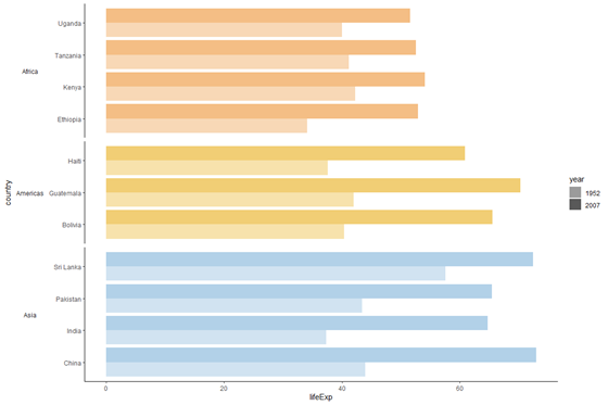
To reduce chartjunk, let'southward suppress the legend for continent because we already have that data in the facets. We will use the guides() part to suppress the legend for the fill aesthetic (recall that nosotros set up aes(fill = continent) in geom_bar()).
          # remove the legend for "fill"
            plot_nolegend <- plot_facet_clean + guides(fill = Faux)               # display the plot object
              plot_nolegend
DataNovia has an excellent guide for formatting ggplot legends, if you lot'd like to modify the fable further e.1000. alter its position, manually change legend colours, etc.
Graph labels
Finally, permit'due south use the labs function to alter the labels for this graph. We want to:
- Remove the ten-axis label — nosotros don't need to say "state" since it is credible
- Change the y-axis label to "Life expectancy (years)"
- Add a title above the graph explaining what the graph shows
- Add together the information source below the graph
          # change graph labels
            plot_final <- plot_nolegend +
            # remove x-axis label
            xlab("") +
            # change the y-axis label
            ylab("Life expectancy (years)") +
            # add together caption and title
            labs(title = "Life expectancy in select countries in 1952 and 2007",
            caption = "Data source: Gapminder")               # display the plot object
              plot_final
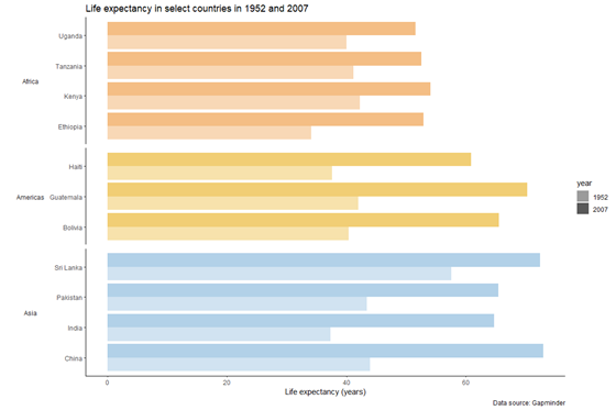
And that is our graph!
Concluding graph code
Here is all the graph code in 1 identify:
          ## base plot
            ggplot(data = data_graph, aes(x = land, y = lifeExp)) +                 ## change the theme
              # utilize basic black and white theme - this theme removes the groundwork color past default
              theme_bw() +
              # remove gridlines. panel.filigree.major is for verical lines, console.filigree.minor is for horizontal lines
              theme(panel.filigree.major = element_blank(), panel.grid.minor = element_blank(),
              # remove borders
              panel.border = element_blank(),
              # removing borders too removes x and y axes. Add them dorsum
              centrality.line = element_line()) +                                         ## add bars
              geom_bar(stat = "identity", aes(fill up = continent, alpha = year), position = "dodge") +
              scale_fill_manual(values = c("#F4BE85", "#F1CE75", "#B2D1E8")) +
              scale_alpha_manual(values = c(0.half dozen, 1)) +                                         ## make the plot horizontal
              coord_flip() +                                         ## add together facets
              facet_grid(rows = vars(continent), scales = "free_y", space = "free_y", switch = "y") +
              # move facet label outside the chart expanse i.e. continent names should be to the left of country names
              theme(strip.placement = "outside",
              # remove background colour from facet labels
              strip.background  = element_blank(),
              # remove edge from facet label
              panel.border = element_blank(),
              # make continent names horizontal
              strip.text.y = element_text(angle = 180)) +                                         ## remove legend
              guides(fill = FALSE) +                                         ## modify graph labels
              # remove x-axis label
              xlab("") +
              # change the y-centrality label
              ylab("Life expectancy (years)") +
              # add caption and championship
              labs(title = "Life expectancy in select countries in 1952 and 2007",
explanation = "Information source: Gapminder")
You can save a copy of the graph using the ggsave() command, which allows you to specify the save location, dimensions of the file, image format (.png, .jpg etc.), and more.
Revisiting ggplot() graph components
Now that we sympathize how to build a ggplot, let's map the elements of our graph to the components of a plot:
- "A default dataset and fix of mappings from variables to aesthetics" — nosotros did this in
ggplot(data = data_graph, aes(10 = country, y = lifeExp)). - "1 or more layers, with each layer having one geometric object, one statistical transformation, one position aligning, and optionally, one dataset and ready of aesthetic mappings"— we created a layer for bars using
geom_bar(),stat = "identity"and "position = "dodge". - "I scale for each aesthetic mapping used" — the ten and y axes had default scales based on the values of "country" and "lifeExp". We also created scales for
fillandalpha. - A coordinate organisation — Cartesian, in our instance, as nosotros specified aesthetics for
10andy. We besides flipped the axes. - The facet specification — we did this using
facet_grid().
The graph components are succinctly expressed in this code template:
          ggplot(information = <DATA>,
            mapping = aes(<MAPPING>)) +
            <GEOM_FUNCTION>(
            stat = <STAT>,
            position = <POSITION>
            ) +
            <COORDINATE_FUNCTION> +
            <FACET_FUNCTION>
Next steps
You lot tin can make the following graphs to learn more nearly ggplot():
- Modify the font and font size for the chart championship, facet labels, and axis labels (y'all'll need to use the
theme()function) - Modify the existing graph to show the value of life expectancy for each bar (you'll need to add a
geom_text()) - Create some dummy data with conviction intervals for estimates of life expectancy, and bear witness these confidence intervals on our existing graph (yous'll need to use
geom_errorbar()) - Create a line graph showing the value of life expectancy over several years for dissimilar countries (you'll demand to utilise
geom_line()and take a new subset of the data) - Y'all tin can have a expect at the ggplot2 cheatsheet to become more ideas for what you can do!
Nosotros would love to know if this worked for you. Write to united states of america with questions or share your graphs with us in the comments below.

Source: https://medium.com/idinsight-blog/how-to-make-bar-graphs-using-ggplot2-in-r-9812905df5d2
Posted by: rutledgepaus1952.blogspot.com
0 Response to "How To Arbitrarily Label Draws In R"
Post a Comment